GSoC 2015
It had been quite an awesome thing to be selected in Google Summer of Code for the second time. Along with it, I also got an offer to pursue masters in Johns Hopkins University in Computer Science in upcoming Fall. The god has been great to me! I thank almighty for all this .
Okay, back to work.
So my project this year deals with implementing "Approximate algorithms for inference in graphical models" in the awesome org. pgmpy. I will try to encompass everything that I have understood till now by reading various research papers and the help I had from the mentors in the form of naive questions. (I think I may need to keep the post updating. Below is what I have understood till now.)
What are graphical models?
A graphical model is a probabilistic model where the conditional dependencies between the random variables are specified via a graph. Graphical models provide a flexible framework for modelling large collections of variables with complex interactions.
In this graphical representation, the nodes correspond to the variables in our domain, and the edges correspond to direct probabilistic interactions between them
Graphical models are good in doing the following things:
- Model Representation
- It allows tractable representation of the joint distribution.
- Very transparent
- Inference
- It facilitates answering queries using our model of the world.
- For example: algorithms for computing the posterior probability of some variables given the evidence on others.
- Say: we observe that it is night and the owl is howling. We wish to know how likely a theft is going to happen, a query that can be formally be written as P(Theft=true | Time=Night, Conditions=Owl is howling)
- Learning
- It facilitates the effective construction of these models by learning from data a model that provides a good approximation to our past experience
- They sometimes reveal surprising connections between variables and provide novel insights about a domain.
Why we want to do inference? Ahem!! What is this "inference" actually!
The fundamental inference problem underlying many applications of graphical models is to find the most likely configuration of the probability distribution also called as the MAP (Maximum a Posteriori) assignment. This is what the underlying problem is while solving the stereo vision and protein design problems.
The graphical models that we consider involve discrete random variables. And it is known that a MAP inference can be formulated as an integer linear program.
There are many ways to solve the MAP inference problem namely:
- Message Passing Algorithms: They solve the inference problem by passing messages along the edges of the graph that summarize each variable's beliefs. Better check Yedidia et al., 2005 paper for a gentle introduction in message propagation. However, these algorithms can have trouble converging, and in difficult inference problems tend not to give good results
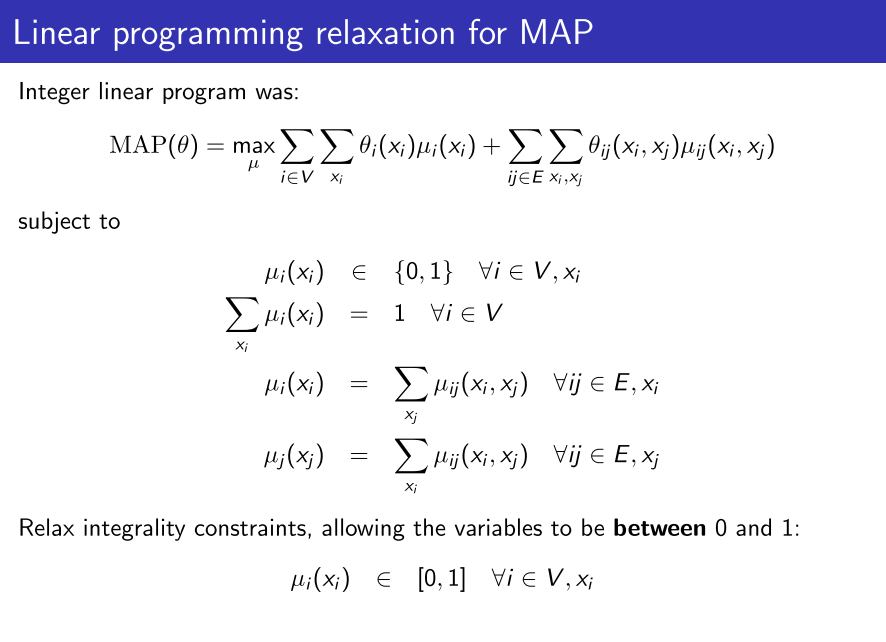
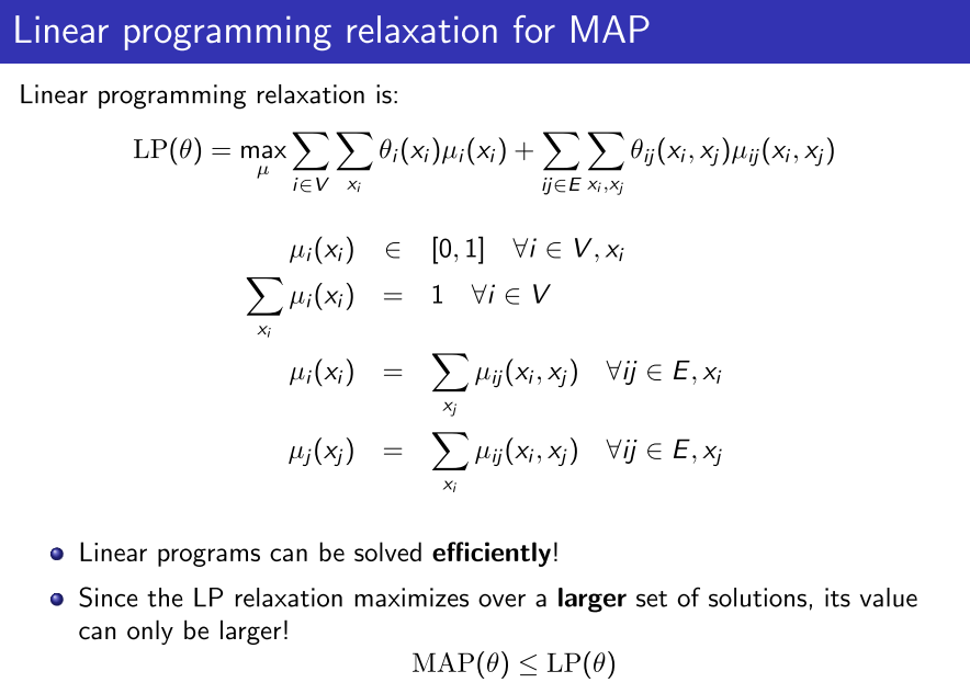
- LP Relaxation: The LP relaxation is obtained by formulating inference as an integer linear program and then relaxing the integrality constraints on the variables. (More on this later!)
To correctly find the MAP assignment is equivalent to finding the assignment $latex x_m&s=2$ that maximizes
$latex \theta(x) = \Sigma_{ij \in E}\theta_{ij}(x_i, x_j)+\Sigma_{i \in V} \theta_i(x_i)&s=3$
To understand what the above term is, we need to delve into the theory of pairwise Markov Random Fields. For the moment being, think of $latex \theta_{ij}&s=2$ as the edge potential and $latex \theta_{i}&s=2$ as the vertex potential.
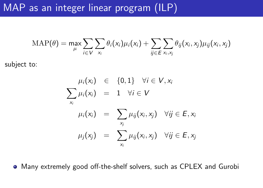
To turn the above into an integer linear program( ILP ), we introduces variables
- $latex \mu_i(x_i)&s=1$, one for each $latex i \in V&s=1$ and state $latex x_i&s=1$
- $latex \mu_{ij}(x_i, x_j)&s=1$, one for each edge $latex ij \in E&s=1$ and pair of states $latex x_i, x_j&s=1$
The objective function is then:
$latex \max_{\mu} \Sigma_{i \in V}\Sigma_{x_i}\theta_{i}(x_i) \mu_i(x_i)+\Sigma_{ij \in E}\Sigma_{x_i, x_j}\theta_{ij}(x_i, x_j) \mu_{ij}(x_i, x_j)&s=3$
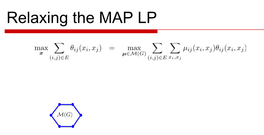
The set of $latex \mu&s=1$ that arises from such joint distributions is known as the marginal polytope. There always exist a maximizing $latex \mu&s=1$ that is integral- a vertex of the marginal polytope - and which corresponds to $latex x_m&s=1$
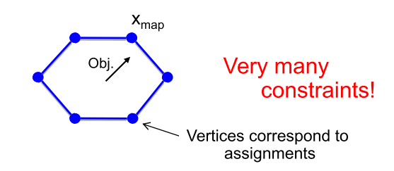
Although the number of variables in this LP is less, the difficulty comes from an exponential number of linear inequalities typically required to describe the marginal polytope.
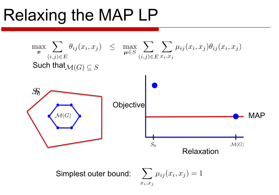
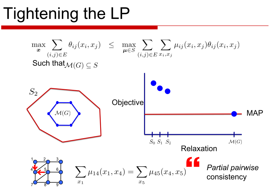
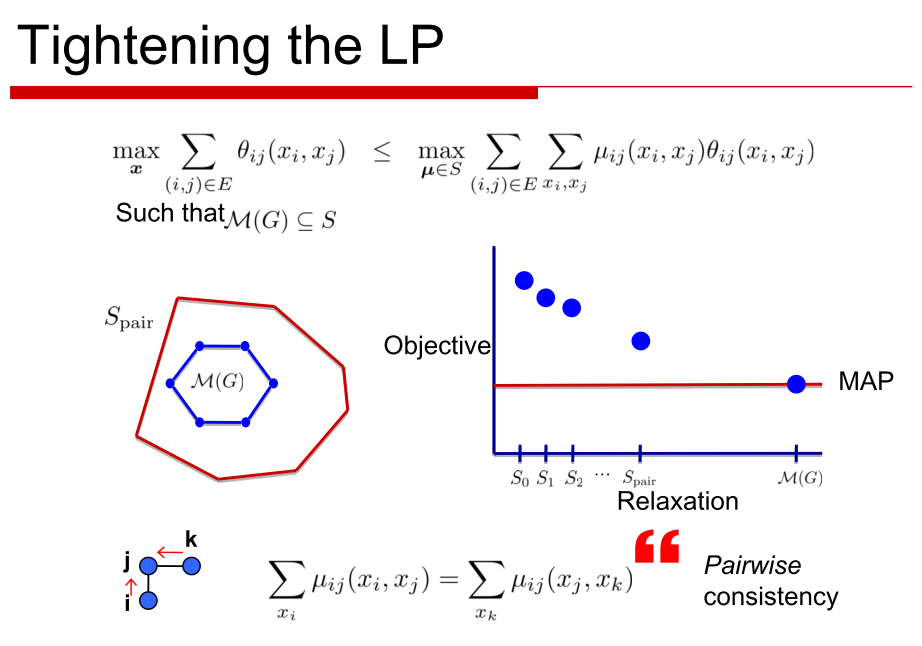
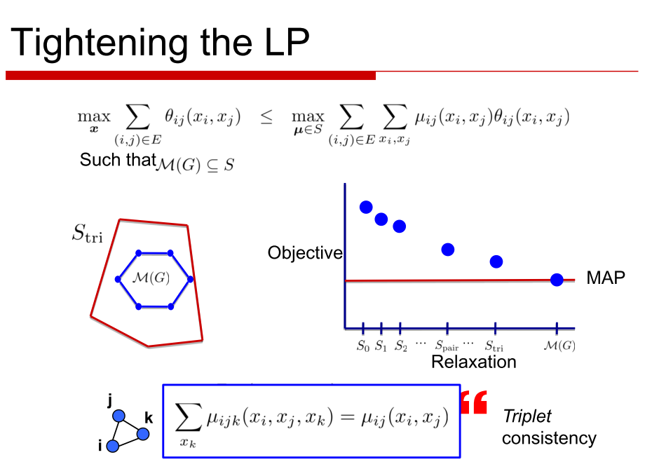
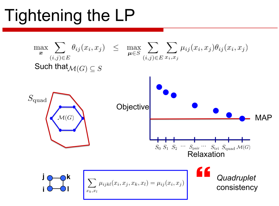
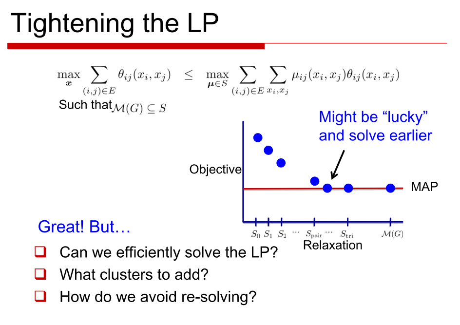
The idea in LP relaxations is to relax the difficult global constraint that the marginals in $latex \mu$ arise from some common joint distribution. Instead we enforce this only over some subsets of variables that we refer to as clusters.
But what are constraints? How come you can use constraints and clusters interchangeably?
What constraint is to Marginal Polytope is clusters to the primal LP problem.
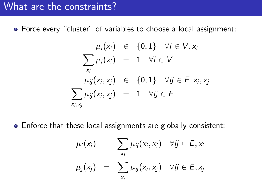
So essentially, we here force every "cluster" of variables to choose a local assignment instead of enforcing that these local assignments are globally consistent. Had these local assignments been consistent globally, we would have the complete Marginal Polytope already.
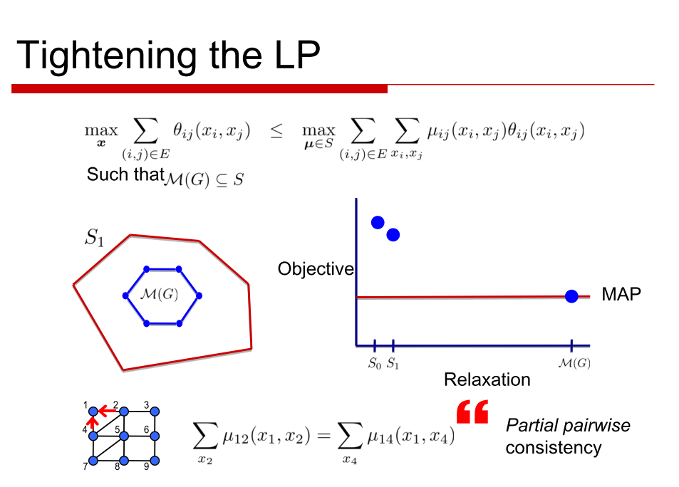
We slowly and steadily add each of the clusters so that we tend towards the Marginal Polytope.
I am attaching few slides that I have found really useful in this case:
Through LP relaxation we solve for the case where the fewer clusters were assigned the local assignment( The local consistency polytope).The solution to this gives us the equation mentioned in the last above.
Why we need approximate algorithms? Is there any other way to do it like exact ones? If exact ones are there, why not use them!!
Solving for the marginal polytope gets too heavy. I will showcase the process in the form of some other slides that I really found useful.
What are the types of approximate algorithms that you are going to implement? Are there many types?
LP Relaxation is the obvious one that is my target here. The other one above where I have added constraints to the marginal polytope is called the cutting plane method ( It happens to be a specific algorithm used in LP Relaxations to tend towards the MAP polytope)
Please describe step by step process of these algorithms. How does approximations helps when accuracy is concerned. Tell about the trade-offs that happen between accuracy and speed!
*I will get onto it soon*
Do previous implementation of what you are going to do already exists? If they, how you plan to make your implementation different from them. Is the language different?
I think they do exist in OpenGM library. I will surely take inspiration out of it. Yup, It is in C++ and we were to make our implementation in Python.
YOU MUST CHECK OUT THE AWESOME LIBRARY I AM WORKING WITH: Pgmpy
